Reuse code with functions

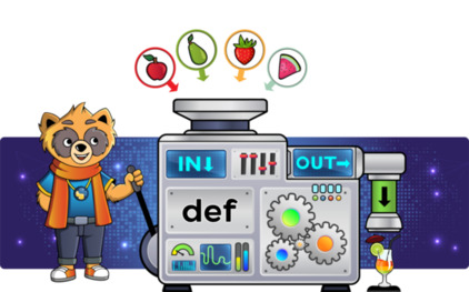
Functions allow us to group and reuse code, abstracting complexity for the user. It does not matter what is inside; you simply need to know what goes in and what comes out. Every function has:

• 📩 Input arguments: What enters the function.
• 📤 Output arguments: What comes out of the function.
• 📑 Code: Defines the behavior, indicating how the inputs are transformed into the outputs.

Next, we will see how to define functions with def, the difference between pass-by-value and reference, the use of decorators with @, generators with yield, asynchronous functions with async, and lambda functions with lambda.

Introduction to functions

Functions are a set of instructions grouped under a name. They are defined with def and have a name, input parameters, and an output.

def sum(a, b):
    result = a + b
    return result

There are other variants, such as functions that do not return any arguments or functions that do not accept any input arguments. Thanks to functions, we can:

• ♻️ Reuse: Eliminate repetitive code. Instead of writing the same 10 lines repeatedly, you can put them in a function and call it when needed in one line.
• 📦 Organize: Group related code together, making it easier to understand. Instead of having a huge block of code doing multiple things, it is better to divide it into functions with specific functionality.
• ⬛ Abstract: Abstract the complexity inside. A function can be very complex internally, but it is enough for the user to know what inputs it accepts and what outputs it returns. This is the well-known black box approach. It does not matter what is inside; it only matters to know what goes in and what comes out.

Let’s look at a function that converts degrees Celsius to Fahrenheit.

def celsius_to_fahrenheit(celsius):
    fahrenheit = (celsius * 9/5) + 32
    return fahrenheit

The function can be called with (), passing in the necessary arguments and capturing what it returns in a temperature_f variable.

temperature_c = 25
temperature_f = celsius_to_fahrenheit(temperature_c)
print(temperature_f)
# 77.0

We can also simplify the function to one line.

def celsius_to_fahrenheit(celsius):
    return (celsius * 9/5) + 32

Since Python is neither statically typed nor compiled, if we call our function with a str, we will get the following error. This is because the divide operation is not defined for str and int. It makes sense, you cannot divide text by 5.

The interesting thing here is that the error is not detected until the function is called. It is a runtime error.

print(celsius_to_fahrenheit("text"))
# TypeError: unsupported operand type(s)

An important note is that it is not the same to use the function with and without ().

• With (): This calls the function with some input arguments.
• Without (): This accesses the function itself, which is an object of the function class.

# With ()
print(celsius_to_fahrenheit(30))
# 86.0

# Without ()
print(celsius_to_fahrenheit)
# <function celsius_to_fahrenheit at 0x1009341f0>

Functions also accept various input parameters.

import math

def hypotenuse(a, b):
    return math.sqrt(a**2 + b**2)

print(hypotenuse(3, 4))
# 5.0

We can call the function by indicating the name of the argument, which is equivalent.

print(hypotenuse(a=3, b=4))
# 5.0

Since the arguments are named, we can also change the order.

print(hypotenuse(b=3, a=4))

As expected, if we pass the name of an argument that does not exist, we will get an error.

print(hypotenuse(c=10))
# TypeError: hypotenuse()

The arguments of a function can also have a default value. This will be used if none is passed. In this case, if b is not passed, it will take 1 as the default value.

def multiply(a, b=1):
    return a * b

print(multiply(10))
# 10

print(multiply(10, 2))
# 20

It is important that the arguments with default values go after those without, otherwise we will get an error. This definition is not correct.

def multiply(a=1, b):
    return a * b

# SyntaxError

On the other hand, functions can have a variable number of arguments, using *args.

def sum(*args):
    return sum(args)

This sum function can be called as follows.

print(sum())
# 0

print(sum(100, 200))
# 300

print(sum(5, 3, 2, 2, 2))
# 12

And if you want to name each argument, you can do it like this.

def sum(**kwargs):
    total = 0
    for key, value in kwargs.items():
        print(key, value)
        total += value
    return total

print(sum(a=5, b=20, c=23))
# 48

print(sum(a=1, b=2))
# 3

Similarly, we can pass a dictionary as an input parameter. It is equivalent to the above.

d = {'a': 5, 'b': 20, 'c': 23}
print(sum(**d))
# 48

We can also have functions that accept a number of fixed parameters (arg1 and arg2) and other variables (args). The following function allows between 2 and n arguments.

def variable_arguments(arg1, arg2, *args):
    print(f"Fixed arguments: {arg1}, {arg2}")
    print(f"Variable arguments: {args}")

With 0 arguments, we get an error, since arg1 and arg2 are mandatory.

variable_arguments()
# TypeError:

Using 2 arguments.

variable_arguments(1, 2)
# Fixed arguments: 1, 2
# Variable arguments: ()

Using 4 arguments.

variable_arguments(1, 2, 3, 4)
# Fixed arguments: 1, 2
# Variable arguments: (3, 4)

But it does not end there. We can also have a variable number of arguments to which we can give a name. The function below combines all types of arguments:

• Two positional fixed arguments: arg1 and arg2. These must always be present.
• Positional variable arguments: *args. We can pass as many as we want.
• Variable key/value arguments: **kwargs. We can also pass as many as we want, but they must be named.

def variable_arguments(arg1, arg2, *args, **kwargs):
    print(f"Fixed arguments: {arg1}, {arg2}")
    print(f"Variable arguments: {args}")
    print(f"Key/value arguments: {kwargs}")

Let’s see an example of how to use it.

variable_arguments(1, 2, 3, 4, other_arg=10, more_arg=20)
# Fixed arguments: 1, 2
# Variable arguments: (3, 4)
# Key/value arguments: {'other_arg': 10, 'more_arg': 20}

Having seen the input arguments, let’s look at the output arguments. A function can have multiple output arguments. This function calculates the mean and variance of some data.

def mean_and_variance(data):
    mean = sum(data) / len(data)
    variance = sum((x - mean) ** 2 for x in data) / len(data)

    return mean, variance

print(mean_and_variance([10, 20, 30, 40]))
# (25.0, 125.0)

As you can see, a tuple is returned. If you want to assign the values to different variables, you can do the following.

mean, variance = mean_and_variance([10, 20, 30, 40])
print(mean)     # 25.0
print(variance) # 125.0

Imagine that you do not want the variance. You can ignore it by using _.

mean, _ = mean_and_variance([10, 20, 30, 40])

On the other hand, a function without an explicit return will automatically return None. The following function returns nothing, but Python automatically returns None.

def my_function():
    pass

output = my_function()
print(output)
# None

It is important to be aware of this because it can lead to hours of wasted time looking for where the None is coming from. In some cases, it may be more difficult to notice.

def time_to_meal(hour):
    match hour:
        case 8:
            return "Breakfast"
        case 14:
            return "Lunch"
        case 21:
            return "Dinner"

print(time_to_meal(7))
# None

Therefore, it is better to be explicit and take into account the None. The result is the same, but it is more explicit.

def time_to_meal(hour):
    match hour:
        case 8:
            return "Breakfast"
        case 14:
            return "Lunch"
        case 21:
            return "Dinner"
        case _:
            return None

print(time_to_meal(7))
# None

Functions can also be assigned to variables. In this case, say_hello acts as an alias for greet.

def greet(name):
    return f"Hello, {name}!"

say_hello = greet

And we can call it.

print(say_hello("John"))
# Hello, John!

Functions can also be stored in a list. In this case, we store add and subtract in operations.

def add(x, y):
    return x + y

def subtract(x, y):
    return x - y

operations = [add, subtract]
print(operations[0](10, 5)) # 15
print(operations[1](10, 5)) # 5

A function can also return another function by storing a context, in this case the factor. This is known as a closure. It is just a function with another function inside plus some context.

def create_multiplier(factor):
    def multiply(x):
        return x * factor
    return multiply

multiply_by_2 = create_multiplier(2)
multiply_by_3 = create_multiplier(3)

print(multiply_by_2(5)) # 10
print(multiply_by_3(5)) # 15

A function can also be an input argument to another. Inside the function, we can call the other one. You can see how execute calls function.

def execute(function, a, b):
    return function(a, b)

def add(a, b):
    return a + b

print(execute(add, 3, 4))
# 7

As you can see, you can do anything with functions. This is because Python treats functions as objects of the function class.

def add(a, b):
    return a + b

print(type(add))
# <class 'function'>

And as a last note, it is a good practice that your functions do not have side effects. That is, they do not modify external variables. This example is not ideal. The function modifies an external variable.

i = 0

def increment():
    global i
    i += 1
    return i

print(increment()) # 1
print(increment()) # 2
print(increment()) # 3

Pass by value and reference

In many programming languages, there are two ways to pass input arguments to a function:

• 📋 By value: A local copy of the variable is created. Any modification on it will have no effect on the original one.
• 🔗 By reference: The input variable is modified directly. Modifications will affect the original variable.

📋 Let’s look at an example of pass by value. As you can see, x does not change. The function acts on a copy and does not modify the original value.

x = 10
def function(input):
    input += 1

function(x)
print(x)
# 10 <- The x does NOT change

🔗 Now let’s look at an example of passing by reference. As you can see, x changes. The function acts directly on x.

x = [10]
def function(input):
    input.append(20)

function(x)
print(x)
# [10, 20] <- The x DOES change

This difference can be somewhat complicated to understand in Python, since it is not possible to explicitly indicate whether we want it to be treated by value or by reference as in other languages.

The key difference is that the first example uses an int and the second uses a list. The behavior is defined by the type of variable used:

• 📋 Immutable types such as int or string are passed as a value. The function cannot modify the original variable.
• 🔗 Mutable types such as list are passed as a reference. The function modifies the original value.

When in doubt, we can use id() to know if two variables refer to the same variable. We can see how the id() is different.

📋 Pass by value. The id is different. They are different variables. Modifying one does not modify the other.

x = 10
def function(input):
    input += 1
    print(id(input)) # 4341262928

print(id(x)) # 4341262960
function(x)

🔗 Pass by reference. The id is the same. It is the same variable. If you modify one, the other is also modified.

x = [10]
def function(input):
    input.append(20)
    print(id(input)) # 4299629568

print(id(x)) # 4299629568
function(x)

You can see, therefore, how in Python the behavior of passing by value or by reference is directly related to mutable and immutable data types. As a final note, let’s look at some advantages and disadvantages of these types:

• 📋 Immutable: Data is protected from modification, which makes it more secure. However, it may require more memory, as they are continuously being copied.
• 🔗 Mutable: The original data can be modified. They require less memory, since the original variable is used, without having to copy it. It is very useful when working with types that store a lot of data, where it would not be feasible to copy continuously.

Documenting functions

Code is read more times than it is written. It is important to document it well so that other people can understand it. Although it sounds obvious, the reality is that documenting is something that is done little and poorly.

To document functions, it is important to apply the black box approach. It does not matter what is inside, but what goes in and what comes out.

Simple programs can be documented in the following way. It is not the best way, but it serves the purpose. You will find millions of functions documented this way. It is the simplest.

def add(a, b):
    # Takes two numbers and returns their sum
    return a + b

However, Python offers docstrings (PEP257). A more correct way to document. This is a docstring in a function. It is defined using """. They can also be used in classes, modules, or methods.

def add(a, b):
    """Take two numbers and return their sum."""
    return a + b

Unlike comments with #, the docstrings are accessible at runtime using __doc__.

print(add.__doc__)
# Take two numbers and return their sum

And similarly with help().

help(add)
# Help on function add in module __main__:
#
# add(a, b)
# Takes two numbers and returns their sum

Although the above comment is perfectly valid, if we create more complex functions or develop open source libraries, we may need to include more information.

There are different ways. Google recommends doing it this way. A description of the function, the input arguments with their type, and the output arguments are included.

def add(a, b):
    """
    Returns the sum of two numbers.

    Args:
        a (int, float): The first number to add.
        b (int, float): The second number to add.

    Returns:
        int, float: The sum of a and b.
    """
    return a + b

Another way is according to the reStructuredText format. This allows us to generate documentation automatically with tools like sphinx. Having the documentation next to the code makes it easier to keep it up to date.

def add(a, b):
    """
    Returns the sum of two numbers.

    :param a: The first number to add.
    :type a: int, float
    :param b: The second number to add.
    :type b: int, float
    :return: The sum of a and b.
    :rtype: int, float
    """
    return a + b

Also, numpy has its own way of doing it, and there are dozens of variations. But no matter which one, they all give similar information with different formatting.

As a final note:

• If you contribute to open source, it is advisable to use English to document your functions. You will be able to reach more people with your packages.
• Not all functions need 50-line comments following a standard. For simple functions, one line is enough. Choose according to your case.

Type annotations

Python has dynamic typing, which means that variables do not have to be defined with a specific type before using them. The type is determined at runtime based on its value.

The arguments of a function do not have a specific type; a and b can be of any type. Other languages such as Go or C require us to determine the exact type.

def multiply(a, b):
    return a * b

This makes Python a very flexible but also dangerous language. The following calls work, but the second one returns a result that we might not have expected.

print(multiply(2, 5))
# 10

print(multiply("2", 5))
# 22222

But the following gives an error, since multiplying two str is not defined.

print(multiply("2", "2"))
# TypeError

To avoid this kind of error at runtime, Python offers type annotations (PEP 3107). They are a kind of metadata associated with the input and output arguments of functions.

In other words, it allows you to tell people using your code what kind of data they should use as input.

# script.py
def multiply(a: int, b: int) -> int:
    return a * b

But they are not enforced. That is, even if we say that a and b are expected to be int, the following code can be executed just as before. The error is obtained at runtime.

print(multiply("2", "2"))
# TypeError

Fortunately, there are tools like mypy that allow detecting this type of incorrect call before the code is executed. It is some kind of static type checker.

mypy script.py

And in our case, it will tell us.

# error: Argument 1 to "multiply" has incompatible type "str"; expected "int"
# error: Argument 2 to "multiply" has incompatible type "str"; expected "int"

You can also access these annotations using the following.

print(multiply.__annotations__)
# {'a': <class 'int'>, 'b': <class 'int'>}

These annotations can be used at runtime. You can create a function that makes sure that a and b are int and raises an error otherwise. You can define any logic you want.

def multiply(a: int, b: int) -> int:
    annotations = multiply.__annotations__
    if not isinstance(a, annotations['a']):
        raise TypeError(f"a must be int, not {type(a)}")

    if not isinstance(b, annotations['b']):
        raise TypeError(f"b must be int, not {type(b)}")

    return a * b

print(multiply("2", "2"))
# TypeError: a must be int, not <class 'str'>.

There is an annotation for each type, and you can mix them with default values.

def power(base: float, exponent: int = 2) -> float:
    return base ** exponent

It also allows you to specify more complex types. This function takes a dict that uses str as key and str as value and returns a list of int.

from typing import List, Dict

def process(cfg: Dict[str, str]) -> List[int]:
    # ...

A summary of the benefits of annotations:

• 📝 Documentation: They make reading easier by clearly indicating what type of data the function expects.
• ✅ Validation: Tools like mypy can use the annotations to check that the types are correct. This way, we avoid surprises at runtime with things that can be prevented earlier.
• ✨ Autocomplete: Editors like PyCharm and VSCode can take advantage of annotations to improve autocompletion and code navigation.

Although you will see a lot of code without annotations, it is advisable to use them. We recommend that you do so from now on.

Recursion with functions

Recursion is a concept in programming where a function calls itself a finite number of times. This allows us to solve problems that can be broken down into smaller subproblems, similar to the original problem.

An example is the calculation of the factorial n!. This operation consists of multiplying a number by all the previous ones. The factorial 4! is 4*3*2*1 = 24. It is a problem that can be solved recursively because:

• Computing 4! involves computing 3! and multiplying by 4.
• Computing 3! involves computing 2! and multiplying by 3.
• Computing 2! involves computing 1! and multiplying by 2.
• The factorial 1! is always 1.

We can express this in code as follows. As you can see, the factorial function calls itself. On each new call, the value of n is reduced by 1.

def factorial(n):
    # recursive
    if n == 1:
        return 1
    else:
        return n * factorial(n-1)

Any recursive function has two well-identified branches:

• 🔁 Recursive call: The function calls itself. It is common for the new call to be made by making some modification to the input. In the case of the factorial, n-1.
• ✋🏼 Return: At some point, the function stops calling itself and returns. This branch is important because if it does not exist, the function could enter an infinite loop.

Although recursion is fine, do not forget that this can also be written in the normal way. The following code calculates the factorial but without recursion.

def factorial(n):
    # non-recursive
    result = 1
    for i in range(2, n+1):
        result *= i
    return result

Another example is to calculate the Fibonacci series. This series calculates the element n by adding the two previous ones, being the first two 0 and 1. As you can see, the next element is the sum of the two previous ones.

# 0, 1, 1, 2, 3, 5, 8, 13, 21, 34

Similar to the factorial, we can calculate the n element as follows.

def fibonacci(n):
    # recursive
    return n if n <= 1 else fibonacci(n-1) + fibonacci(n-2)

And we can also express it non-recursively like this. Again, with loops of all life.

def fibonacci(n):
    # non-recursive
    a, b = 0, 1
    for _ in range(n):
        a, b = b, a + b
    return a

Another interesting example of recursion is to convert a list of n dimensions into 1 dimension, something known as flatten.

In this case, we have a list with lists inside. The goal is to have a single list without nesting. This example is interesting since it mixes recursion with generators, something we will see later.

def flatten(lst):
    for item in lst:
        yield from flatten(item) if isinstance(item, list) else (item,)

nested_list = [1, [2, [3, 4], 5], 6]
print(list(flatten(nested_list)))
# [1, 2, 3, 4, 5, 6]

Decorating functions

Decorators are functions that allow us to modify the behavior of other functions. If you have seen a function preceded by @, that is a decorator.

Let’s see an example. We are going to create a decorator that shows the time it took to execute a function. The decorator is defined with def, as if it were a normal function.

The decorator accepts as input a func function and returns it with slightly modified behavior.

import time

# This is a decorator
def measure_time(func):
    def wrapper(*args, **kwargs):
        t0 = time.time()
        res = func(*args, **kwargs)
        print(f"{func.__name__}: {time.time() - t0:.5f} seconds")
        return res
    return wrapper

Now we can use our decorator with @measure_time on any function. For example, the following function determines whether a number is prime or not.

The only change is that it now prints the time it took to run. The rest is the same.

# This is using a decorator
@measure_time
def is_prime(n):
    return n > 1 and all(n % i != 0 for i in range(2, int(n**0.5) + 1))

print(is_prime(99999999999973))
# is_prime: 0.56682 seconds
# True

That is, we have modified the behavior of the function without actually changing it. We have decorated it.

You can also modify the function to return other arguments. In this case, we return the time it took to execute as well as whether it is prime or not.

def measure_time(func):
    def wrapper(*args, **kwargs):
        t0 = time.time()
        # We return the result
        # and the time it took
        return func(*args, **kwargs), time.time() - t0
    return wrapper

Although both examples are valid, there is an important nuance. If we look at the function metadata, it refers to the decorator, not the decorator of our function. For example.

# the decorator has changed the metadata
print(is_prime.__name__)
# wrapper

If we want to preserve metadata, such as name and documentation, a good practice is to use wraps as follows. It is common to see decorators defined in this way.

from functools import wraps
import time

def measure_time(func):
    @wraps(func)
    def wrapper(*args, **kwargs):
        t0 = time.time()
        return func(*args, **kwargs), time.time() - t0
    return wrapper

If you now access the name, you can see how it is maintained.

# With wraps now the metadata does not change
print(is_prime.__name__)
# is_prime

On the other hand, it is also possible to pass parameters to our decorators. Just as a function can have input arguments and default values.

Let’s see an example with a decorator that tries to execute a function multiple times in case it fails. We have two parameters:

• 🔁 retries: Defines the number of times the function is attempted to be executed. After this number of attempts, it is considered to have failed.
• 💤 backoff_seconds: Waiting time between consecutive attempts. It is important to define this because if a call fails, if we try without waiting, we may encounter the same error. Waiting a bit between attempts usually increases the chances of success.

This decorator can be useful when we have functions that can sometimes fail. It will allow us to try again when it fails up to a maximum number of times.

def retry(retries, backoff_seconds=1):
    def decorator(func):
        @wraps(func)
        def wrapper(*args, **kwargs):
            for attempt in range(1, retries + 1):
                try:
                    print(f"Attempt {attempt}")
                    return func(*args, **kwargs)
                except Exception as e:
                    print(f"Error: {e}")
                    if attempt == retries:
                        raise e
                    time.sleep(backoff_seconds)
        return wrapper
    return decorator

Now we can use our decorator in the following way. With random, we try to reproduce a function that can fail with a probability of 30%. Imagine this is a request to an external server or database.

You can see how if failure occurs, it tries again up to a maximum number of 3 times, waiting 2 seconds between attempts.

@retry(retries=3, backoff_seconds=2)
def function_fail():
    import random
    if random.random() < 0.7:
        raise ValueError("Random error")
    print("Completed")

Yield and generators

Generators and yield were introduced in PEP255. Their use returns a lazy iterator. Next, we will see what lazy means.

A lazy iterator does not store the values in memory. It allows them to be generated “on the fly.” Hence its name. It does not store them. Let’s see two examples:

• [: Creates a list of 1000 items. This is NOT lazy.
• (: Creates a generator of 1000 elements. This is lazy.

not_lazy = [i for i in range(1000)] # NOT lazy
is_lazy = (i for i in range(1000))  # IS lazy

At first glance, it might seem that they are the same since the result of the following code is identical.

for i in not_lazy: print(i)
for i in is_lazy: print(i)

However, they are two different things. The type of the first is list and the second generator.

print(type(not_lazy)) # <class 'list'>
print(type(is_lazy))  # <class 'generator'>

We can see that the size they occupy in memory is different. Here we have the first advantage of lazy iterators. They hardly occupy any memory.

import sys
print(f"a: {sys.getsizeof(not_lazy)} bytes")
# a: 8856 bytes

print(f"b: {sys.getsizeof(is_lazy)} bytes")
# b: 112 bytes

But there are disadvantages. The generator cannot be indexed.

print(not_lazy[50]) # 50
print(is_lazy[50])  # TypeError

The generator cannot be iterated twice.

for i in is_lazy: pass
for i in is_lazy: print(i)

Having seen the differences, let’s get down to practicalities. Generators allow us to generate values on demand. This allows us to save resources. As you have seen, generators consume a fixed amount of memory. The disadvantage is that the values are not there but are generated as they are needed.

This is very useful when you work with very large data and files. It is common that when you open a file, like the open() function, you are not loading the whole file into memory but creating a kind of generator. This allows you to iterate the file, but it is not loaded into memory. It is loaded as needed.

We have seen how to create a generator with ( using list comprehensions, but you can also create it using yield.

def my_generator():
    yield 0
    yield 1
    yield 2

As you can see, it is a generator.

print(type(my_generator()))
# <class 'generator'>

And you can use them as follows.

for i in my_generator():
    print(i)
# 0, 1, 2

Since a generator is an iterator, we can manually access the following element

g = my_generator()
print(next(g)) # 0
print(next(g)) # 1
print(next(g)) # 2

When you get to the end, you will get StopIteration. That is, at the 4 time you call next.

print(next(g)) # StopIteration

For example, you can create a prime number generator. First, we define is_prime to find out if a number is prime.

def is_prime(n: int) -> bool:
    return n > 1 and all(n % i != 0 for i in range(2, int(n**0.5) + 1))

And we create our prime number generator. Notice that we use yield. Whenever you think of generators, think of yield.

def primes(n):
    num, counter = 2, 0
    while counter < n:
        if is_prime(num):
            yield num
            counter += 1
        num += 1

In this example, we generate the first 5 prime numbers. The advantage of this is that they are generated as needed.

for p in primes(5):
    print(p)
# 2, 3, 5, 7, 11

In addition, there are many generator-friendly functions such as sum(), any(), all(), min(), max(), map(), filter(), or enumerate() among others. This is very useful since they allow working with the generator data without having to load all its elements in memory.

For example, we can add the first 100000 prime numbers with sum() using our generator.

print(sum(primes(100000)))
# 62260698721

Finally, we can use a list comprehension as we have seen above, but using generators. An example:

• We generate the first 1000 prime numbers.
• We square each one **2.
• We add all with sum.

x = sum(x**2 for x in primes(100))
print(x)
# 8384727

Lambdas and functional programming

We can define lambda functions as anonymous functions. More informally, they are quick functions to define if you are too lazy to define a normal one. They can be declared in one line and do not even need to be assigned to a variable. This is a lambda function.

lambda a, b: a + b

It contains two arguments, a and b, and returns their sum. It is optional, but you can assign it to a variable to name it.

add = lambda a, b: a + b

Once we have the function, it is possible to call it as if it were a normal function. As you can see, they are equivalent to the “normal” functions we have seen before.

add(2, 4)

Lambda functions are closely related to functional programming. This is a programming paradigm where everything revolves around functions. It is often said that these are first-class citizens.

In functional programming, it is common to use the following primitives, which are applied to iterables such as lists:

• 🔧 map: Modifies each element.
• 🧲 filter: Filters the elements that meet a condition.
• 🌪️ reduce: Accumulates all the elements, reducing them to a value with a given logic.

Let’s see these three functions in action combined with lambda functions. Imagine we have the following list.

nums = [1, 2, 3, 4, 5]

🔧 With map, we can modify each element using a lambda function. We modify each element by squaring it.

But there is a trick to it. What is returned is not the modified list. It is an iterator.

print(map(lambda x: x**2, nums))
# <map object at 0x1046ff940>

Since it is an iterator, you can iterate over it in the following way. This is closely related to generators and the concept of lazy seen earlier.

for i in map(lambda x: x**2, nums):
    print(i)
# 1, 4, 9, 16, 25

If you want to get the list, you can convert the iterator to list.

nums_squared = list(map(lambda x: x**2, nums))
print(nums_squared)
# [1, 4, 9, 16, 25]

So far, nothing new. You can get the same result with the same old loops.

nums_squared = []
for x in nums:
    nums_squared.append(x**2)
print(nums_squared)
# [1, 4, 9, 16, 25]

🧲 With filter, we can filter the values. For example, we keep the even numbers.

nums_even = list(filter(lambda x: x % 2 == 0, nums))
print(nums_even)
# [2, 4]

Which is equivalent to doing the following.

nums_even = []
for x in nums:
    if x % 2 == 0:
        nums_even.append(x)

print(nums_even)
# [2, 4]

🌪️ And with reduce, we can accumulate all values into one. For example, we add them all together.

from functools import reduce

total = reduce(lambda x, y: x + y, nums)
print(total)
# 15

Which is equivalent to this.

total = 0
for x in nums:
    total += x
print(total)
# 15

As you can see, map, filter, and reduce allow us to do things we already knew how to do but in a different way. It avoids loops and is closer to how it would be done in functional programming.

There is also a small nuance. Both map and filter are lazy, which means that they return an iterator that computes values as needed, applying our function to each element. This consumes very little memory.

The case of reduce is different since it uses eager evaluation. That is, it calculates the resulting value.

Although we have previously used map with lambda functions, we can also use normal functions. Although they require a few more lines of code.

def square(x):
    return x ** 2

nums_squared = list(map(square, nums))
print(nums_squared)
# [1, 4, 9, 16, 25]

Finally, let’s look at a practical example. We have a list of people with different attributes.

people = [
    {'Name': 'Alice', 'Age': 22, 'Gender': 'F'},
    {'Name': 'Bob', 'Age': 25, 'Gender': 'M'},
    {'Name': 'Charlie', 'Age': 33, 'Gender': 'M'},
    {'Name': 'Diana', 'Age': 15, 'Gender': 'F'},
    {'Name': 'Esteban', 'Age': 30, 'Gender': 'M'},
]

We can keep everyone’s names.

names = list(map(lambda p: p['Name'], people))
print(names)
# ['Alice', 'Bob', 'Charlie', 'Diana', 'Esteban']

Or we can filter out those over 32 years old.

seniors_32 = list(filter(lambda p: p['Age'] > 32, people))
print(seniors_32)
# [{'Name': 'Charlie', 'Age': 33, 'Gender': 'M'}]

We can also sort by age and keep the names. We can see that Diana is now first.

sorted_names = list(
    map(lambda x: x["Name"],
    sorted(people, key=lambda p: p['Age'])))
print(sorted_names)
# ['Diana', 'Alice', 'Bob', 'Esteban', 'Charlie']

This is one of the interesting things about Python. It is a multi-paradigm programming language, which means that we can do the same thing in very different ways. In this section, we have seen how to do it in a more functional way.

Asynchronous functions

So far, we have seen code and functions that are executed sequentially. In order. One instruction after another. Until one function is finished, the next one does not start.

However, this can be inefficient. Imagine a function that makes a request to an external server on the other side of the world. This request may take a few seconds. What do we do in the meantime? Wait and do nothing?

This is not efficient since this external request is blocking our program. Until the server responds, we will be waiting without doing anything. We can use this time to do other tasks.

Luckily, Python provides us with tools for asynchronous programming, where our program can continue to run while waiting. This is widely used in:

• 🕸️ Web scraping.
• 💽 Databases.
• 📁 Input and output with files.
• 🖥️ Graphical interface development.

In all these cases, at some point, we are blocked waiting for an external response. Next, we will see the differences between:

• 🐌 Synchronous programming: The traditional model seen so far, where we finish the previous task to execute the next one.
• 🏎️ Asynchronous programming: When a task blocks us, we continue executing others, allowing us to perform multiple tasks “in parallel.”

🐌 Let’s look at a synchronous example. The following code creates 10 processes. Imagine that the sleep simulates the time it takes for an external service to respond. This program takes 10 seconds to execute. Until one process is finished, the next one is not started.

import time
def process(process_id):
    time.sleep(1)
    print("End process:", process_id)

[process(i) for i in range(10)]

🏎️ Let’s see an asynchronous example using asyncio. In this case, when it detects that we are blocked, it continues executing other code. Therefore, all 10 processes are started at the same time, and after 1 second, everything is completed. We have gone from 10 seconds to 1.

import asyncio

async def process(process_id):
    await asyncio.sleep(1)
    print("End process:", process_id)

async def main():
    await asyncio.gather(*[process(i) for i in range(10)])

asyncio.run(main())

It is important to note that in this case, the order is not guaranteed. Even less so if we depend on something external whose response time can be variable. The use of await indicates where we should wait.

On the other hand, there are packages such as threading that allow similar tasks to be performed, although with a completely different concurrency model, beyond the scope of this book.

It is often useful when working with libraries that do not support async and allows you to take advantage of a multi-core CPU. Note that it does not offer parallel execution due to GIL.

import threading
import time

def process(process_id):
    time.sleep(1)
    print("End process:", process_id, flush=True)

threads = [threading.Thread(target=process, args=(i,)) for i in range(10)]
[i.start() for i in threads]
[i.join() for i in threads]

There is also the multiprocessing package, which does offer parallel execution, and we can benefit from multiple CPUs. This library is useful for computationally intensive tasks such as multiplying very large matrices.

from multiprocessing import Process
import time

def process(process_id):
    time.sleep(1)
    print(f"End process: {process_id}", flush=True)

def main():
    processes = [Process(target=process, args=(i,)) for i in range(10)]
    [p.start() for p in processes]
    [p.join() for p in processes]

if __name__ == '__main__':
    main()