Monte Carlo simulation with numpy

In this example, we perform a Monte Carlo simulation on an investment portfolio using numpy. This type of simulation is common for investment portfolios, which involve the following parameters:

• 💶 An initial amount of money.
• 📈 An expected but not fixed annual return, which varies according to volatility.
• ❓ A volatility factor that causes the annual return to fluctuate.
• ⏳ A time span of several years.

The objective is to calculate the final amount of money after the specified time period. If volatility were 0 and the annual return were fixed each year, the calculation would be straightforward. However, financial markets are subject to uncertainty.

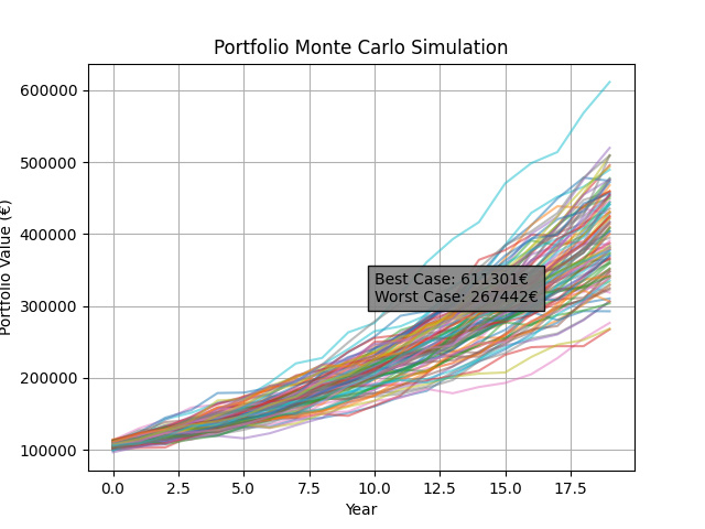
We can model this uncertainty with Monte Carlo methods, examining different possible scenarios to gain insight into the best and worst cases.

We simulate this volatility with a normal distribution using np.random.normal. Once we have it, we calculate the portfolio_value over the years and plot it on a graph.

import numpy as np
import matplotlib.pyplot as plt

def simulate_portfolio(initial, annual_return, annual_volatility, time_years, simulations):
    np.random.seed(42)
    returns = np.random.normal(annual_return, annual_volatility, (time_years, simulations))
    portfolio_value = initial * (1 + returns).cumprod(axis=0)

    plt.figure()
    plt.plot(portfolio_value, alpha=0.5)
    plt.title("Portfolio Monte Carlo Simulation")
    plt.xlabel("Year")
    plt.ylabel("Portfolio Value (€)")
    plt.grid(True)

    best_case = portfolio_value.max(axis=1)[-1]
    worst_case = portfolio_value.min(axis=1)[-1]
    plt.text(time_years / 2, best_case / 2,
             f'Best Case: {best_case:.0f}€\nWorst Case: {worst_case:.0f}€',
             bbox=dict(facecolor='grey', alpha=0.9))

    plt.show()

Now, we can use the function with the following parameters. We perform 100 simulations over a 20-year horizon, expecting an annual return of 7% with a volatility of 4%, starting with 100,000 Euros.

simulate_portfolio(
    initial=100_000,
    annual_return=0.07,
    annual_volatility=0.04,
    time_years=20,
    simulations=100)

This simulation provides insight into the potential outcomes for the portfolio, illustrating both the best and worst cases. As you can see, none of our simulations resulted in a loss after 20 years.

✏️ Exercises:

• Perform the simulation using different combinations of annual_return and annual_volatility. Identify a combination that results in losses in some scenarios.
• Add a new representation showing the average of all possible scenarios on a single line. That is called the ensemble average.